Random Numbers and Probability

import pandas as pd
import numpy as np
import matplotlib.pyplot as plt

Random Numbers and Probability

This Random Numbers and Probability is part of Datacamp course: Introduction to Statistic in Python

Here we’ll explore how to generate random samples and measure chance using probability.We will work with real-world sales data to calculate the probability of a salesperson being successful. Finally, we will try to use the binomial distribution to model events with binary outcomes.

This is my learning experience of data science through DataCamp

Measuring chance

\[ P(\text{event}) = \frac{\text{# ways event can happen}}{\text{total # of possible outcomes}} \]

Sampling with replacement vs sampling without replacement

sampling without replacement, in which a subset of the observations are selected randomly, and once an observation is selected it cannot be selected again. sampling with replacement, in which a subset of observations are selected randomly, and an observation may be selected more than once

Calculating probabilities

You’re in charge of the sales team, and it’s time for performance reviews, starting with Amir. As part of the review, you want to randomly select a few of the deals that he’s worked on over the past year so that you can look at them more deeply. Before you start selecting deals, you’ll first figure out what the chances are of selecting certain deals.

Recall that the probability of an event can be calculated by

\[ P(\text{event}) = \frac{\text{# ways event can happen}}{\text{total # of possible outcomes}} \]

amir_deals = pd.read_csv('amir_deals.csv', index_col=0)
amir_deals.head()

	product	client	status	amount	num_users
1	Product F	Current	Won	7389.52	19
2	Product C	New	Won	4493.01	43
3	Product B	New	Won	5738.09	87
4	Product I	Current	Won	2591.24	83
5	Product E	Current	Won	6622.97	17

counts = amir_deals['product'].value_counts()
print(counts)

# Calculate probability of picking a deal with each product
probs = counts / len(amir_deals['product'])
print(probs)

Product B    62
Product D    40
Product A    23
Product C    15
Product F    11
Product H     8
Product I     7
Product E     5
Product N     3
Product G     2
Product J     2
Name: product, dtype: int64
Product B    0.348315
Product D    0.224719
Product A    0.129213
Product C    0.084270
Product F    0.061798
Product H    0.044944
Product I    0.039326
Product E    0.028090
Product N    0.016854
Product G    0.011236
Product J    0.011236
Name: product, dtype: float64

Sampling deals

In the previous exercise, you counted the deals Amir worked on. Now it’s time to randomly pick five deals so that you can reach out to each customer and ask if they were satisfied with the service they received. You’ll try doing this both with and without replacement.

Additionally, you want to make sure this is done randomly and that it can be reproduced in case you get asked how you chose the deals, so you’ll need to set the random seed before sampling from the deals.

# Set random seed
np.random.seed(24)

# Sample 5 deals without replacement
sample_without_replacement = amir_deals.sample(5,replace=False)
print(sample_without_replacement)

       product   client status   amount  num_users
128  Product B  Current    Won  2070.25          7
149  Product D  Current    Won  3485.48         52
78   Product B  Current    Won  6252.30         27
105  Product D  Current    Won  4110.98         39
167  Product C      New   Lost  3779.86         11

# Set random seed
np.random.seed(24)

# Sample 5 deals with replacement
sample_with_replacement = amir_deals.sample(5,replace=True)
print(sample_with_replacement)

       product   client status   amount  num_users
163  Product D  Current    Won  6755.66         59
132  Product B  Current    Won  6872.29         25
88   Product C  Current    Won  3579.63          3
146  Product A  Current    Won  4682.94         63
146  Product A  Current    Won  4682.94         63

Discrete distributions

• Probability distribution
  • Describe probability of each possible outcome in a scenario
  • Expected value: mean of probability distribution
• Law of large number (LLN): as size of sample increases, sample mean will approach expected value.

Creating a probability distribution

Restaurant management wants to optimize seating space based on the size of the groups that come most often to a new restaurant. One night, 10 groups of people are waiting to be seated at the restaurant, but instead of being called in the order they arrived, they will be called randomly. This exercise examines the probability of picking groups of different sizes.

Remember that expected value can be calculated by multiplying each possible outcome with its corresponding probability and taking the sum

restaurant_groups = pd.read_csv('restaurant_groups.csv')
restaurant_groups.head()

	group_id	group_size
0	A	2
1	B	4
2	C	6
3	D	2
4	E	2

# Create a histogram of restaurant_groups and show plot
restaurant_groups['group_size'].hist(bins=[2, 3, 4, 5, 6])

<AxesSubplot:>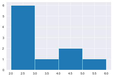

# Create probability distribution
size_dist = restaurant_groups['group_size'].value_counts() / restaurant_groups.shape[0]
# Reset index and rename columns
size_dist = size_dist.reset_index()
size_dist.columns = ['group_size', 'prob']
print(size_dist)

# Expected value
expected_value = np.sum(size_dist['group_size'] * size_dist['prob'])
print(expected_value)

# Subset groups of size 4 or more
groups_4_or_more = size_dist[size_dist['group_size'] >=4]

# Sum the probabilities of groups_4_or_more
prob_4_or_more = groups_4_or_more['prob'].sum()
print(prob_4_or_more)

   group_size  prob
0           2   0.6
1           4   0.2
2           6   0.1
3           3   0.1
2.9000000000000004
0.30000000000000004

Continuous distributions

Data back-ups

Your company’s sales software backs itself up automatically, but no one knows exactly when the back-ups take place. It is known, however, that back-ups occur every 30 minutes. Amir updates the client data after sales meetings at random times. When will his newly-entered data be backed up? Answer Amir’s questions using your new knowledge of continuous uniform distributions

from scipy.stats import uniform

# Min and max wait times for back-up that happens every 30 min
min_time = 0
max_time = 30

# Calculate probability of waiting less than 5 mins
prob_less_than_5 = uniform.cdf(5, min_time, max_time)
print(prob_less_than_5)

# Calculate probability of waiting more than 5 mins
prob_greater_than_5 = 1 - uniform.cdf(5, min_time, max_time)
print(prob_greater_than_5)

# Calculate probability of waiting 10-20 mins
prob_between_10_and_20 = uniform.cdf(20, min_time, max_time) - \
                        uniform.cdf(10, min_time, max_time)
print(prob_between_10_and_20)

0.16666666666666666
0.8333333333333334
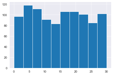
0.3333333333333333

Simulating wait times

To give Amir a better idea of how long he’ll have to wait, you’ll simulate Amir waiting 1000 times and create a histogram to show him what he should expect. Recall from the last exercise that his minimum wait time is 0 minutes and his maximum wait time is 30 minutes.

np.random.seed(334)

# Generates 1000 wait times between 0 and 30 mins
wait_times = uniform.rvs(min_time, max_time, 1000)
print(wait_times[:10])

# Create a histogram of simulated times and show plot
plt.hist(wait_times);
print ("Unless Amir figures out exactly what time each backup happens, he won't be able to time his data entry so it gets backed up sooner, but it looks like he'll wait about 15 minutes on average\n")

[ 7.144097    0.97455866  3.72802787  5.11644319  8.70602482 24.69140099
 23.98012075  3.19592668 25.1985306  17.89048629]
Unless Amir figures out exactly what time each backup happens, he won't be able to time his data entry so it gets backed up sooner, but it looks like he'll wait about 15 minutes on average

The binomial distribution

• Binomial distribution
  • Probability distribution of number of successes in a sequence of independent trials
  • Described by n and p
    • n: total number of trials
    • p: probability of success
  • Expected value: n * p
  • Independence: The binomial distribution is a probability distribution of number of successes in a sequence of independent trials

Simulating sales deals

Assume that Amir usually works on 3 deals per week, and overall, he wins 30% of deals he works on. Each deal has a binary outcome: it’s either lost, or won, so you can model his sales deals with a binomial distribution. In this exercise, you’ll help Amir simulate a year’s worth of his deals so he can better understand his performance.

# Import binom from scipy.stats
from scipy.stats import binom

# Set random seed to 10
np.random.seed(10)

# Simulate a single deal
print(binom.rvs(1, 0.3, size=1))

# Simulate 1 week of 3 deals
print(binom.rvs(3,0.3,size=1))

# Simulate 52 weeks of 3 deals
deals = binom.rvs(3,0.3,size=52)

# Print mean deals won per week
print(np.mean(deals))

print('\nIn this simulated year, Amir won 0.83 deals on average each week')

[1]
[0]
0.8461538461538461

In this simulated year, Amir won 0.83 deals on average each week

Calculating binomial probabilities

Just as in the last exercise, assume that Amir wins 30% of deals. He wants to get an idea of how likely he is to close a certain number of deals each week. In this exercise, you’ll calculate what the chances are of him closing different numbers of deals using the binomial distribution.

# Probability of closing 3 out of 3 deals
prob_3 = binom.pmf(3,3,0.3)
print(prob_3)

# Probability of closing <= 1 deal out of 3 deals
prob_less_than_or_equal_1 = binom.cdf(1,3,0.3)
print(prob_less_than_or_equal_1)

# Probability of closing > 1 deal out of 3 deals
prob_greater_than_1 =1- binom.cdf(1,3,0.3)
print(prob_greater_than_1)

print("\nAmir has about a 22% chance of closing more than one deal in a week.")

0.026999999999999996
0.784
0.21599999999999997

Amir has about a 22% chance of closing more than one deal in a week.

How many sales will be won?

Now Amir wants to know how many deals he can expect to close each week if his win rate changes. Luckily, you can use your binomial distribution knowledge to help him calculate the expected value in different situations. Recall from the video that the expected value of a binomial distribution can be calculated by n*p

# Expected number won with 30% win rate
won_30pct = 3 * 0.3
print(won_30pct)

# Expected number won with 25% win rate
won_25pct = 3 * 0.25
print(won_25pct)

# Expected number won with 35% win rate
won_35pct = 3 * 0.35
print(won_35pct)

print('\nIf Amirs win rate goes up by 5%, he can expect to close more than 1 deal on average each week')

0.8999999999999999
0.75
1.0499999999999998

If Amirs win rate goes up by 5%, he can expect to close more than 1 deal on average each week